Evolution of Radio Receivers – Part 2: The Superheterodyne Architecture Explained

1. Introduction

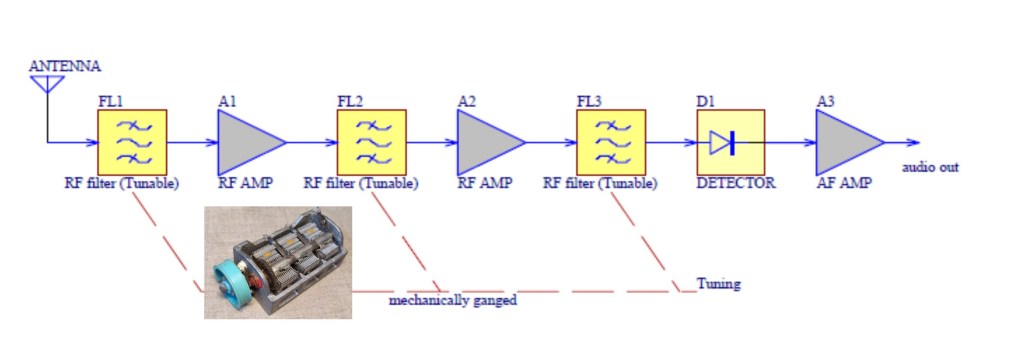
The first commercial radio broadcast began in the 1920s. In the early days, radio receivers were constructed with an antenna feeding a LC tuned circuit which was followed by a simple crystal detector or a vacuum tube amplifying stage and then a diode detector to recover the audio. This is the basic Tuned Radio Frequency (TRF) receiver which was merely adequate when there were only a few stations operating in the 530~1700kHz MW band, also referred to as the Broadcast (BC) Band. As the number of broadcast stations grew, users realized that several stations got mixed together — an indication of poor selectivity. It was also difficult or impossible to receive distant stations because sensitivity was low. Selectivity of a radio receiver is the ability to separate a signal or signals at one frequency from those on all other frequencies. For improvement more LC tuned circuits and amplifying stages were added. A typical TRF receiver of the 1920s has 3 tunable LC circuits tuned to the same frequency. Station selection is accomplished by a 3-gang variable capacitor (as in the photo of fig.1). The block diagram in fig.1 is the ultimate refinement of a TRF receiver.

2. The Problems with TRF receivers

The key feature of an improved TRF receiver is that each of the tuned circuits is isolated by an amplifier so that they do not interact with each other. Such an arrangement is known as a synchronously tuned filter and is the only practical way to increase selectivity in the 1920s when modern filter design theory has not been matured. On the plus side, sensitivity was improved due to the gain provided by the amplifying stages. However two major problems remained: 1. Very difficult or impossible to add more stages to further improve sensitivity. This is because when the total gain is very high, a minuscule portion of the amplified signal at the output may be coupled to the input to cause self-excited oscillation. This phenomenon gets worse as the receiving frequency goes up. 2. Selectivity is uneven across the band. It is best at the low side and worst at the high side, as indicated by the formula or curve in fig.2.

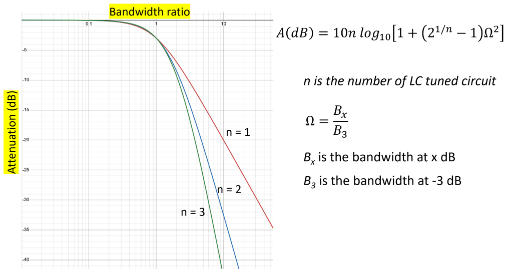
As a numerical example, let’s compare the selectivity of a typical TRF radio with one or three tuned circuits at 3 channel (30kHz) away for a desired receiving frequency of 560kHz and 1500kHz. Assume the loaded Q of the tank circuits is 80.
Case 1: Receiving frequency is 560kHz

• 3dB bandwidth is 560/80 = 7.0kHz for a single LC tuned circuit.
  3dB bandwidth is 560/80*0.51 = 3.6kHz for 3 synchronously tuned LC circuits. (0.51 is the shrinkage factor)
• Bandwidth factor Bx/B3 = 60/7 = 8.6 for a single LC tuned circuit. Bandwidth factor Bx/B3 = 60/3.6 = 16.7 for 3 synchronously tuned LC circuits.
• Selectivity at 3 channel (60kHz) away is -18.7dB for a single LC circuit. Selectivity at 3 channel (60kHz) away is -56dB for 3 synchronously tuned LC circuits.

Case 2: Receiving frequency is 1500kHz

• 3dB bandwidth is 1500/80 = 18.8kHz for a single LC tuned circuit. 3dB bandwidth is 1500/80*0.51 = 9.6kHz for 3 synchronously tuned LC circuits. (0.51 is the shrinkage factor)
• Bandwidth factor Bx/B3 = 60/18.8 = 3.2 for a single LC tuned circuit. Bandwidth factor Bx/B3 = 60/6.4 = 6.25 for 3 synchronously tuned LC circuits.
• Selectivity at 3 channel (60kHz) away is -10.5dB for a single LC circuit.
  Selectivity at 3 channel (60kHz) away is -31.4dB for 3 synchronously tuned LC circuits.

The above example shows that a typical TRF receiver having 3 synchronously tuned LC circuits gives a difference of about 25dB in selectivity between the low and high ends of the MW band. This is very significant and noticeable. Moreover the 3dB bandwidth also differs quite a lot; another undesirable weakness.

When Shortwave (SW) broadcast became popular, the above limitations became gating issues. Edwin Armstrong came up with a highly ingenious and effective solution. He called it the Superheterodyne and obtained a patent for it. The Superheterodyne has several unique advantages that make it the architecture of choice since then.

Regenerative and Super-Regenerative Receivers

Before the superheterodyne became the dominant architecture, radio designers explored other clever ways to overcome the limitations of simple TRF receivers. Two notable approaches that achieved high gain with very few components were the regenerative and super-regenerative circuits. Both relied on positive feedback, but they worked in fundamentally different ways.
Regenerative Receivers
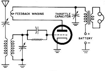
In a regenerative circuit, a small amount of the amplified signal is fed back to the input in phase, dramatically increasing both gain and selectivity. With just one tube or transistor as the RF amplifier, it was possible to achieve surprisingly good sensitivity. The main drawback was its critical nature: highest sensitivity was obtained at the point just before oscillation. Too little feedback produced weak performance, while too much caused the circuit to oscillate, rendering reception impossible. A dedicated control was provided for the user to readjust feedback magnitude after changing frequency; that was a very tedious process. I am not aware of any commercial regenerative receiver in the transistor era. However it remains popular for hobbyists. Fig.3 shows a typical regenerative receiver circuit of the tube era. Note that the “throttle capacitor” sets the amount of positive feedback.

Super-Regenerative Receivers (SRR)
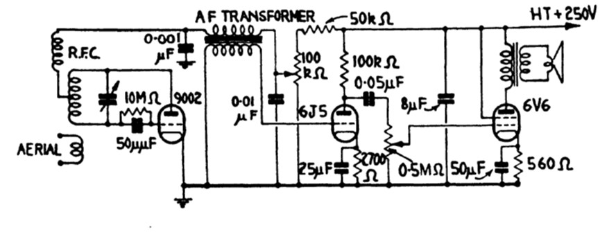
The super-regenerative design has no provision for feedback control. It deliberately let the circuit oscillate but is rapidly “quenched” (turned on and off at an ultrasonic rate, typically 20–50 kHz). This quenching allows the circuit to build up enormous gain during each brief “on” period. This results in extremely high sensitivity. However it suffers from very poor selectivity and high noise levels. It also radiates strongly, causing interference to nearby receivers. As a result super-regenerative design never finds its way in commercial radios. However due to its very low-cost and high sensitivity, it is very popular for toy walkie-talkies, toy remote control models and garage door receivers. Fig.4 is a typical circuit that uses vacuum tubes. I will write another post to describe the SRR in more details.

While regenerative and super-regenerative circuits offered impressive performance for their simplicity, the superheterodyne principle provided a more stable and scalable solution. Interestingly all 3 concepts were conceived or invented by Edwin Armstrong.

From the next section onward we will focus on the superheterodyne architecture.

3. The Superheterodyne Principle

Introduction

Fig. 5 is the block diagram of a typical superheterodyne receiver (superhet for short). The essential blocks of a superhet are the mixer, the local oscillator (LO) and the IF amp. The RF amp (A1) and the tunable filter (FL2) are optional. The key concept of the superhet is to convert the frequency of the input signal to a fixed intermediate frequency (IF) at which filtering and amplification can be done more easily. It is much easier to obtain good selectivity with a fixed frequency filter than with a tunable one. Moreover a stable high gain amplifier is easier to realize at a fixed and lower frequency. Signals picked up by the antenna are filtered by a tunable filter (FL1) which is called the preselector. In the case of no RF amp, The filtered signal goes to the mixer (M1) where it mixes or heterodynes with the signal from the LO. For a MW or SW band radio, the LO is a variable frequency oscillator (VFO).

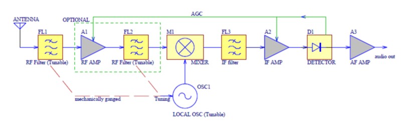
Armstrong’s original invention had a IF of 455kHz which is lower than the lowest frequency of the BC band (530kHz). This is referred to as downconversion and is the scheme used by most receivers in the tube era. For the BC band, the VFO frequency is one IF, i.e., 455kHz above the frequency being received. For example, if 530kHz is to be received, the VFO is tuned to 530+455=985kHz. If 1600kHz is to be received, the VFO must be tuned to 1600+455=2055kHz. This is known as high-side mixing as the LO frequency is greater than the receiving frequency by a IF.

Mixer and Frequency Translation

Mixer is a traditional radio term for a circuit that shifts one signal’s frequency up or down by combining it with another signal. It is more accurately called a frequency mixer to distinguish it from an audio mixer that blends multiple audio inputs for recording or broadcast. Since this blog is dedicated to radio matters, whenever I use the term mixer I am referring to frequency mixer. A mixer works by multiplying the instantaneous voltages of two signals together to produce an output that contains new frequencies. Multiplication is best understood from examination of the following trigonometric identity:

From the above equation, we can observe two important properties:

1. Multiplication results in output signals at the sum and difference frequencies of the input.
2. The amplitude of the IF signal is proportional to the product of the RF and LO amplitudes. If the LO amplitude is constant, the amplitude modulation in the RF signal is transferred to the IF signal.

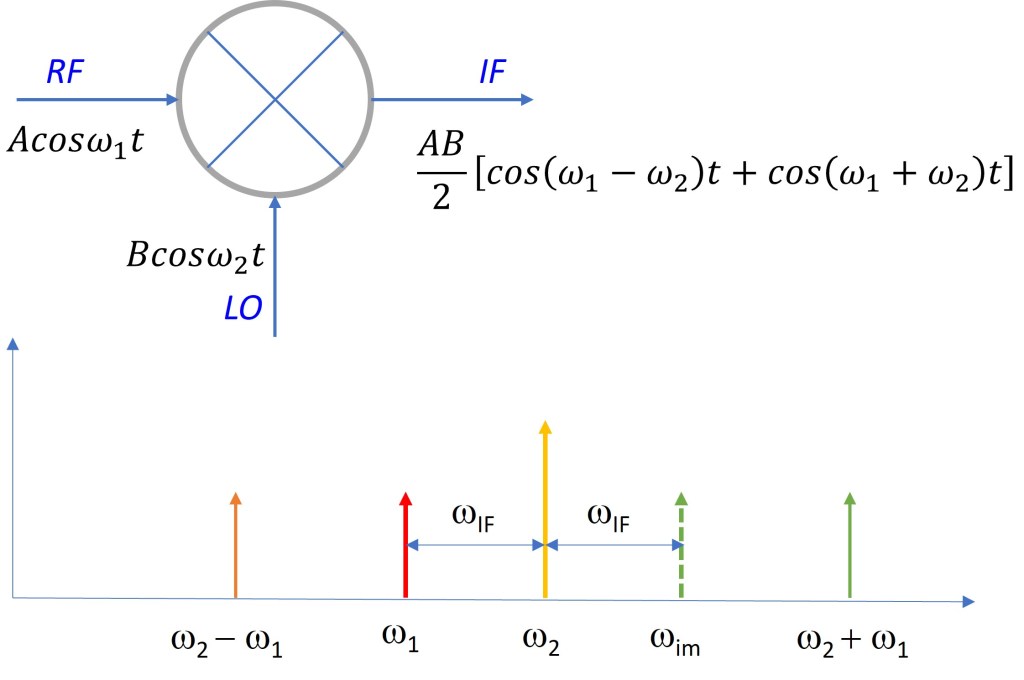
In fig.6 the difference frequency at the output is the intermediate frequency we want; the sum frequency is rejected by the IF filter. Note that there is an image frequency which is higher than the receive frequency by 2 times the intermediate frequency (IF). A signal at the image frequency will be mixed down to produce the same IF and thus causing interference. The image can only be rejected by the preselector filters (FL1 & FL2 in fig.5), or a special image-reject mixer. For a typical MW band radio without a tuned RF stage, image rejection is 35dB at the high-end of the band. It gets worse as the receiving frequency goes up. A higher IF frequency can improve image rejection but destroy adjacent channel selectivity. A 455kHz IF seems a good compromise between selectivity and image rejection for the MW and low SW bands(120m ~ 60m). For higher SW bands, interference from image signals is severe. This gives rise to dual and multiple conversion. More on this later.

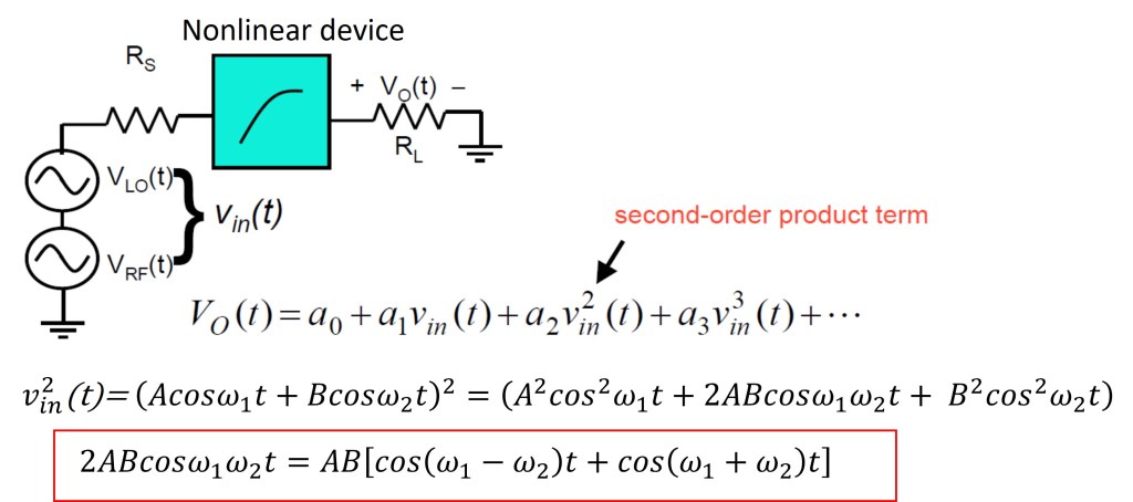
In Armstrong’s original circuit, the mixer was a single vacuum tube, which also served the local oscillator (LO) function. Most if not all portable transistor radios of the 1960s or before employed a single transistor as mixer. Either tube or transistor makes use of their nonlinear transfer characteristics to achieve frequency translation. Such a configuration is known as Single-ended mixer (SEM) which theory is illustrated in fig.7. It must be emphasized that for clarity only the second order term, which produces the desired output, is shown. It is obvious from fig.7 that there are numerous high order mixing products which must be filtered out to avoid interference.

Nowadays there are many different mixer circuit topologies and implementations that perform better than the SEM. I will discuss them in details later in dedicated posts.

Local Oscillator

It is not an overstatement to say that the local oscillator is a critical component of a superheterodyne receiver. Key requirements include frequency stability and phase noise which has great impact on selectivity. The latter was unknown in the early days from tube to early transistor era. Later I will write dedicated posts on phase noise and oscillator design. For the time being, we assume that the LO is an ideal oscillator.

Frequency Converter

For cost reduction, a single transistor (or tube) can function as mixer and local oscillator simultaneously. Most pocket radios use this approach. I will discuss this topic in details in the next post: a classic 6-transistor pocket superheterodyne radio.

Intermediate Frequency (IF) Amplifier

The IF Amplifier provides most of the gain and selectivity of a superheterodyne receiver. The IF filters work on a fixed frequency and are therefore much easier to optimize than the tunable band-pass filters in a TRF receiver. When the superhet was invented, filter synthesis technique was not yet available and hence selectivity at IF was obtained by the so-call synchronously tuned filter, which was implemented by cascading several LC tank circuits each of which was isolated by an amplifying stage. An IF LC tank circuit is called a IF transformers (IFT) because it usually has 2 windings to facilitate inter-stage coupling. Fig.8 is the schematics of a typical 6-transistor AM radio, which is the most used configuration for pocket radios in the 1960s.

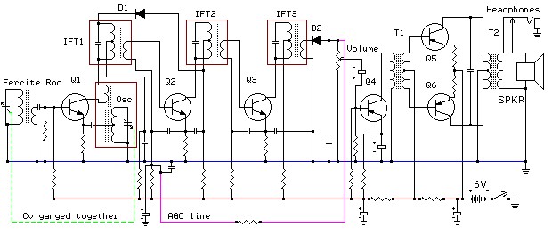
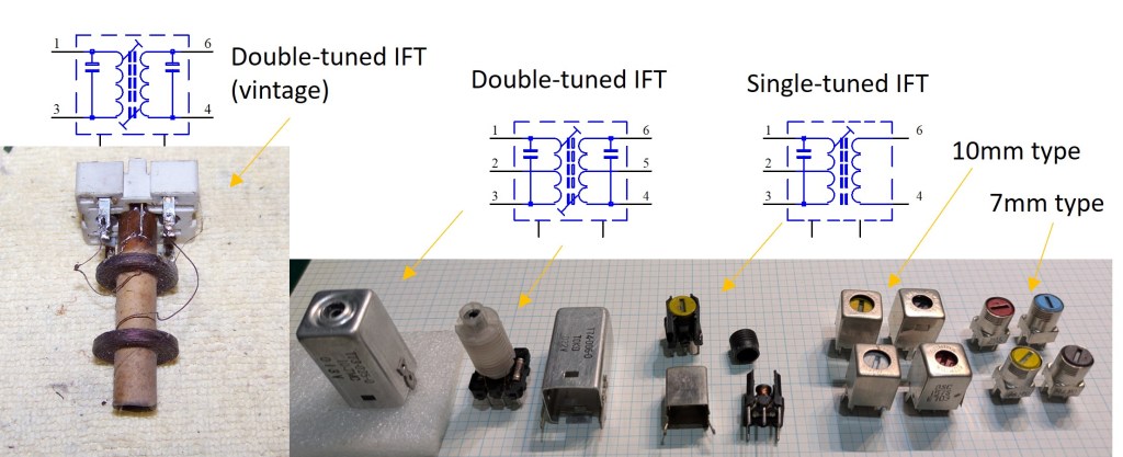
Fig.9 shows some typical IFTs from the early tube era to the present day (from left to right). In the old days, RF inductors or coils had large size and fixed inductance. Tuning was done by adjusting the trimmer capacitors. When high permeability ferrite or powdered-iron materials became available, RF coils could be made smaller and tuned by adjusting the position of the magnetic cores. From early 1960 onward, IFTs were gradually miniaturized and standardized (far right of fig.8).

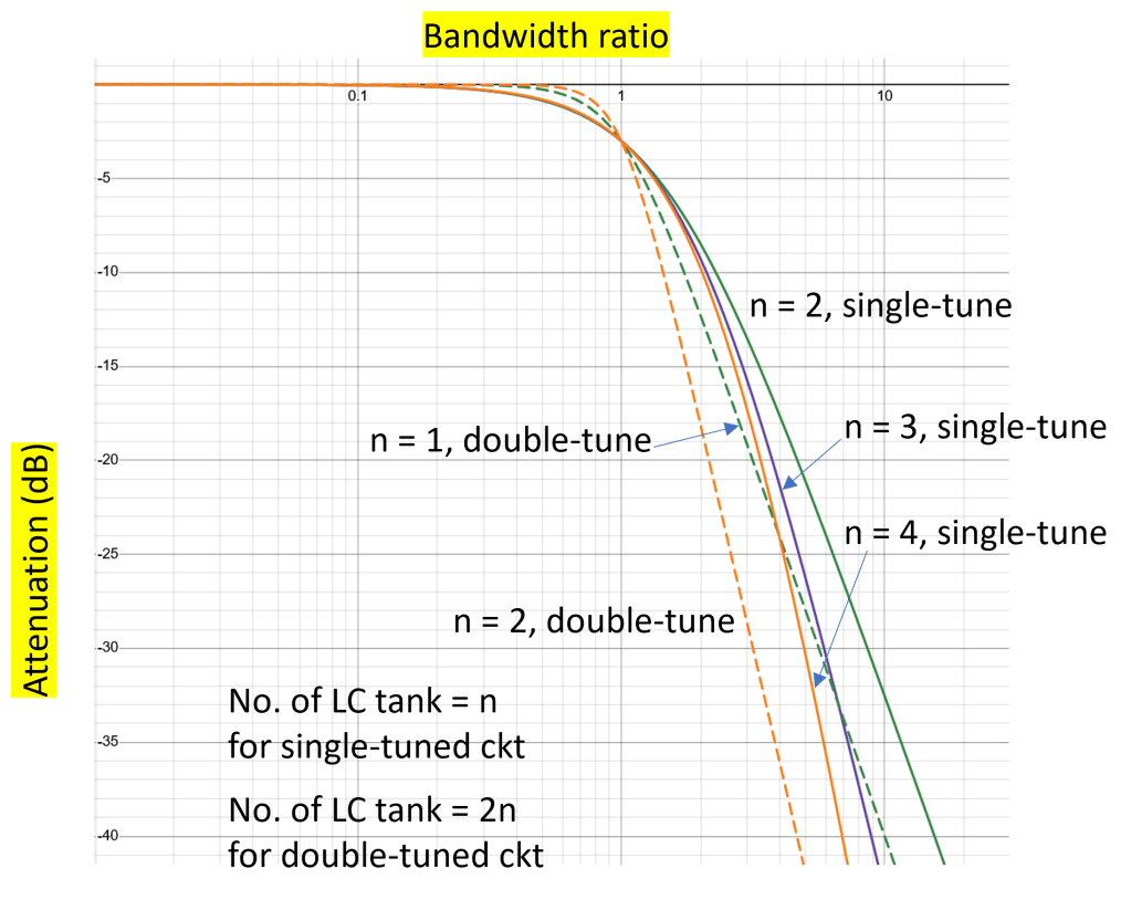
It is interesting to note that almost all tube radios use double-tuned IFTs while most transistor radios use single-tuned IFTs. The major reason is the high input impedance of a tube amplifier that permits a parallel tuned circuit to be connected to its grid. Early transistors are bipolar junction type which have low input impedance. If a LC circuit is connected directly to the base of a transistor, its Q will be loaded down and thus selectivity destroyed. Loading can be reduced but not eliminated by connecting the base of the transistor to a tap of the coil. Most manufacturers did not bother the extra trouble and cost, except for top of the line models or Hi-Fi tuners. Fig.10 compares the selectivity of single and double-tuned circuits. Note that with the same number of LC tanks, for instance, 4 pieces for single-tuned versus 2 pairs for double-tuned, the latter has much better selectivity. Moreover double-tuned circuits have a flatter pass-band (resembling a top-hat) while single-tuned circuits have a narrow bell-like response. In other words, double-tuned circuits retain more high frequency sidebands of the music. Listening tests confirm that tube radios generally have better sound quality. Since the early 1980, even smaller IFTs (5mm and 4mm) were available. However they did not enjoy comparable level of success of the 10mm or 7mm types as high performance and alignment-free ceramic filters became available.

Detector and Automatic Gain Control

The detector for a superhet is basically the same as that for a TRF radio. (Refer to D2 in fig.8.) In the 1960s and 70s, germanium diodes such as 1N34, 1N60, OA47, etc. were used exclusively. From 1980 onward, as Ge diodes became obsolete, silicon diodes such as 1N914, 1N4148 were widely used. The impact on performance, however, was not as obvious as for the TRF radio because the total gain of a superhet was much higher so that the signal at the detector was high enough for a Si diode. As discrete transistors were replaced by integrated circuits, the issue of diode type disappeared as almost all chips had the detector integrated.

Automatic Gain Control (AGC) works by using the DC voltage from the diode detector to alter the bias of the IF amplifier and RF amplifier (if it is used) so as to alter the gain. This works as the gain of a transistor amplifier decreases with lower bias current. Some designs also alter the bias of the transistor mixer. The effect is to obtain a relatively constant audio volume when the received signal fluctuates. In the tube era this is referred to as Automatic Volume Control (AVC).

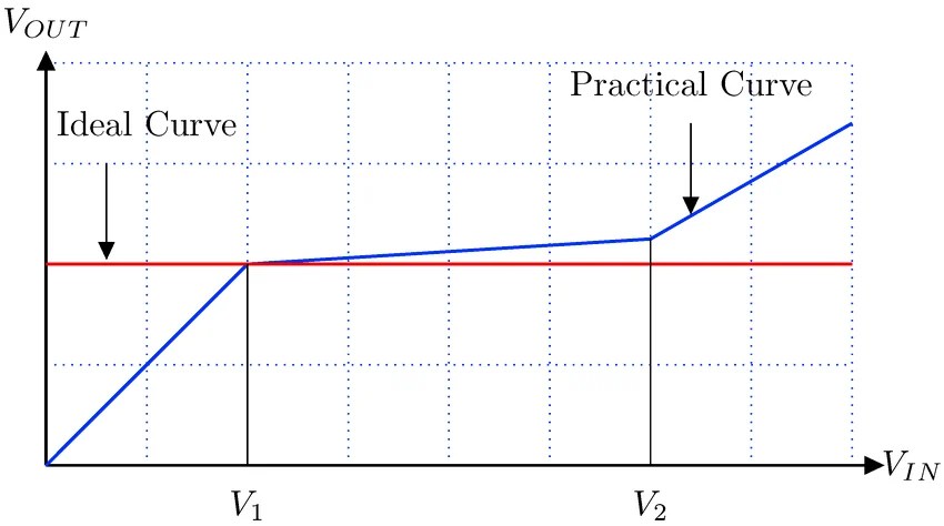
AGC circuitry can be very simple as in a 6-transistor pocket radio (fig.8), where only the first IF amplifier stage is controlled. It can be quite complex in a communications receiver. The AGC Figure of Merit (FOM) quantifies how effectively a receiver maintains a constant output level despite large variations in input signal strength. It is defined as the change in input signal strength (in dB) required to produce a specific, small change in output signal level (usually 1 dB or 2 dB). A higher FOM indicates a more effective AGC action. For example, a high-quality receiver might have an AGC FOM of 100dB, meaning the input can vary by 100dB while the output remains nearly constant. Fig.11 illustrates AGC characteristics.

4. Key Challenges in Superheterodyne Receivers

Although the superheterodyne architecture solved the major limitations of TRF receivers, it introduced its own set of challenges. Understanding these helps explain why the design continued to evolve for decades.

Image Frequency Problem

When the mixer converts the desired radio frequency (RF) to the intermediate frequency (IF), another unwanted frequency — the image frequency — can also mix down to the same IF. For example, if the IF is 455 kHz and you are receiving 1000 kHz, an image at 1910 kHz could also produce a 455 kHz output and cause interference. To suppress the image, a tunable RF bandpass filter known as the preselector is added before the mixer. However, achieving good image rejection across a wide tuning range is not easy. This issue becomes more severe at higher frequencies.

We will explore the image frequency problem in detail, along with advanced solutions such as dual-conversion and triple-conversion superheterodyne architectures, in a future post.

Local Oscillator Tracking

The local oscillator (LO) must always maintain a constant frequency difference (equal to the IF) from the received station as you tune across the band. This requires precise “tracking” between the RF tuning circuit and the LO tuning circuit. Any mismatch causes poor sensitivity or distortion. Early designers used ganged variable capacitors and added padding/tracking capacitors, but achieving perfect tracking over the entire AM or SW band remained a difficult balancing act.

The mathematics and practical techniques of oscillator tracking will be covered in a dedicated future article.

Other Practical Considerations

Additional challenges include managing Automatic Gain Control (AGC) to handle strong and weak signals gracefully, minimizing local oscillator radiation that can cause interference to nearby receivers, and maintaining stability at high frequencies. These issues drove many of the refinements seen in later superheterodyne designs.

Despite these challenges, the advantages far outweighed the difficulties. This is why the superheterodyne principle became the dominant radio architecture for more than 90 years. At present the most advanced DSP/SDR radios still apply the superheterodyne principle.

5. Comparing TRF and Superhet

Feature	TRF Receivers	Superheterodyne Receivers
Selectivity	Poor and frequency-dependent	Excellent and consistent
Bandwidth Control	Difficult (shrinks with more stages)	Easy with fixed IF filters
Gain & Stability	Limited, prone to oscillation	High gain with good stability
Sensitivity	Moderate	Very good
Tuning	Simple but awkward at high frequencies	More complex (tracking required)
Image Rejection	Not applicable	Requires RF preselector
Complexity	Low	Higher, but manageable
Modern Relevance	Mostly obsolete	Still the foundation of most receivers

To Probe Further

We have discussed the principle and building blocks of a superheterodyne radio. With these core concepts understood, we are now ready to look at a practical implementation in Part 3: the classic 6-transistor pocket superheterodyne radio.